Living Museum of Learning
Albert and the Four Spaces of a Tiny Matrix
Today Albert explored Gilbert Strang’s four fundamental spaces using two very small matrices.
The first matrix was:
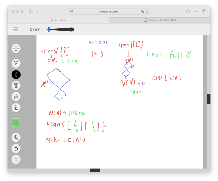
A = [1 2 3]
Even though it is extremely small, it already contains all four fundamental spaces.
Albert first examined the column space of Aᵀ:
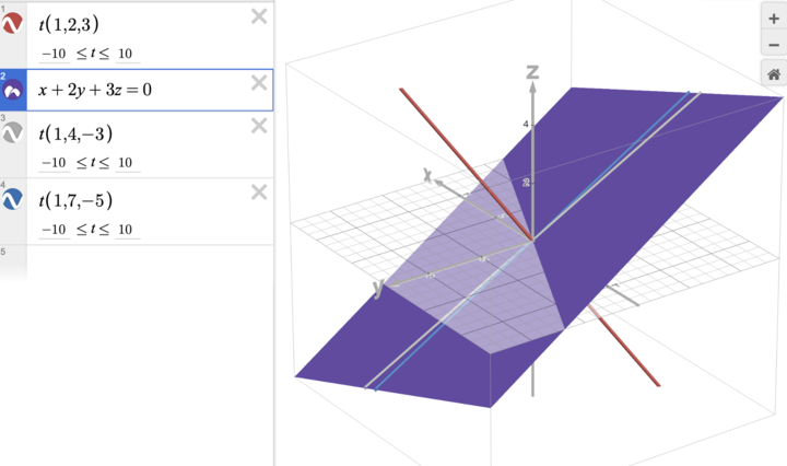
C(Aᵀ) = span{ [1, 2, 3]ᵀ }
Then he solved the homogeneous equation:
x + 2y + 3z = 0
and derived the null space:
N(A) = span{ [1, 4, -3]ᵀ, [1, 7, -5]ᵀ }
He also identified the column space of A:
C(A) = span{ [1] }
and observed that the left null space is trivial:
N(Aᵀ) = {0}
meaning there is no nonzero vector perpendicular to the column space in this case.
---
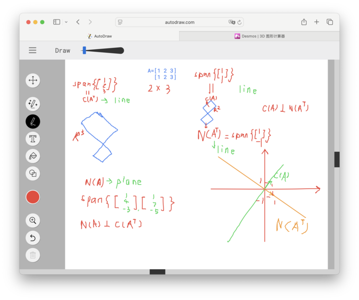
Then Albert changed the structure of the matrix:
A = [1 2 3] [1 2 3]
Now the matrix has two identical rows.
This small change dramatically changes the geometry.
The left null space immediately appears:
N(Aᵀ) = span{ [1, -1]ᵀ }
because the two rows cancel each other:
x + y = 0
This was the key moment: linear dependence creates a new direction in the space of solutions.
Albert could directly see how repeating a row changes rank and introduces new null structure.
---
Through these two tiny matrices, he explored the four fundamental spaces:
• column space • row space • null space • left null space
not as abstract definitions, but as objects that visibly change when the matrix changes.
This is the power of small examples in linear algebra: they make structure observable.
---
Today’s large-scale AI systems, graphics engines, and language models all depend on massive matrix operations.
But the core ideas—rank, dependence, orthogonality, dimension—begin with exactly this kind of simple structure.